Analysis of website text content using quanteda

Introduction to basic text analysis using the quanteda package, in the context of organisational website content.

1. Introduction

In our previous post in this series (Hyperlink networks and website text content), we used tidytext and other packages to conduct text analysis on organisational websites’ content, specifically word frequency counts, word clouds, comparison clouds. In this post, we will demonstrate how to use quanteda to undertake similar text analysis. The post will also introduce some more of the basics of text analysis e.g. constructing a corpus and document-feature matrix and dictionary-based coding. quanteda is an R package for natural language processing and analysis, and tutorials on using quanteda can be found here.

The text content used in this example involves text content from organisational websites involved in the discussion of data sovereignty; these data were collected using rvest (see Hyperlink networks: data pre-processing techniques).

2. Getting the text data ready for analysis

In the first place, we load up the text dataframe that was created in the previous post in this series:

library(dplyr)
library(knitr)

textContent <- readRDS("textContent.rds")
str(textContent)

'data.frame':   75 obs. of  2 variables:
 $ page: chr  "https://womeninlocalization.com/partners/" "https://womeninlocalization.com/data-localization-laws-around-the-world/" "https://iwgia.org/en/network.html" "https://www.iwgia.org/en/indigenous-data-sovereignty/4699-iw-2022-indigenous-data-sovereignty.html?filter_tag[0]=37" ...
 $ text: chr  "Women in Localization (W.L.) is certified as a 501 (c)(3) tax-exempt nonprofit. Its mission is to foster a glob"| __truncated__ " Data localization laws can be a challenge for some and nearly nothing for others. After all, everything depend"| __truncated__ "\r\n\r\n\t\tWritten on 11 March 2011. Posted in About IWGIA\r\n\t Since 1968, IWGIA has worked for protecting, "| __truncated__ "\r\n\r\n\t\tWritten on 01 April 2022. Posted in Indigenous Data Sovereignty\r\n\t Indigenous Peoples have alway"| __truncated__ ...

nrow(textContent)

[1] 75

There are 75 URLs which we used rvest to collect website text content from. In the previous post we noted that a few of these pages are duplicates (http and https versions of the same page) and that there are some URLs that are links to PDF files (from which, rvest does not extract text data). Please note that, to simplify the process we are not pre-processing these issues this exercise.

The next step involves extracting the domain names from the URLs and use a manually-coded .csv file to categorise websites as to whether the represented organisations are based on the Global North or South (see the previous post for more on this).

#function from https://stackoverflow.com/questions/19020749/function-to-extract-domain-name-from-url-in-r
domain <- function(x) strsplit(gsub("http://|https://|www\\.", "", x), "/")[[c(1, 1)]]

dd <- sapply(textContent$page, domain)
textContent$domain <- as.character(dd)

#code websites as from Global North/South
coded <- read.csv("domains_coded.csv")
#> head(coded)
#  X                       x  type
#1 1 womeninlocalization.com north
#2 2               iwgia.org north
#3 3   indigenousdatalab.org north
#4 4           botpopuli.net south
#5 5              cipesa.org south
#6 6              mydata.org north

#now get the north/south classification into the dataframe containing the tokens
textContent$type <- coded$type[match(textContent$domain, coded$x)]

#capitalise the labels, for the plot
textContent$type <- ifelse(textContent$type=="north", "North", "South")

str(textContent)

'data.frame':   75 obs. of  4 variables:
 $ page  : chr  "https://womeninlocalization.com/partners/" "https://womeninlocalization.com/data-localization-laws-around-the-world/" "https://iwgia.org/en/network.html" "https://www.iwgia.org/en/indigenous-data-sovereignty/4699-iw-2022-indigenous-data-sovereignty.html?filter_tag[0]=37" ...
 $ text  : chr  "Women in Localization (W.L.) is certified as a 501 (c)(3) tax-exempt nonprofit. Its mission is to foster a glob"| __truncated__ " Data localization laws can be a challenge for some and nearly nothing for others. After all, everything depend"| __truncated__ "\r\n\r\n\t\tWritten on 11 March 2011. Posted in About IWGIA\r\n\t Since 1968, IWGIA has worked for protecting, "| __truncated__ "\r\n\r\n\t\tWritten on 01 April 2022. Posted in Indigenous Data Sovereignty\r\n\t Indigenous Peoples have alway"| __truncated__ ...
 $ domain: chr  "womeninlocalization.com" "womeninlocalization.com" "iwgia.org" "iwgia.org" ...
 $ type  : chr  "North" "North" "North" "North" ...

Note that there are two domains/organisations for which we do not have a North/South code, but in these two cases there was no text data extracted from the web pages. There is an additional row in the dataframe where the text column is empty. So, we will remove the three domains from our analysis.

#two domains are for web pages where no text data was collected
textContent %>% filter(is.na(type))

                                               page text
1 https://digitallibrary.un.org/record/218450?ln=en     
2                             http://unstats.un.org     
                 domain type
1 digitallibrary.un.org <NA>
2        unstats.un.org <NA>

#we will remove these rows from the dataframe
textContent <- textContent %>% filter(!is.na(type))

#note that there is still one other row in the dataframe where the text column is empty, 
textContent %>% filter(text=="")

                                        page text  domain  type
1 https://doi.org/10.1016/j.jnma.2021.03.008      doi.org North

#so we may as well remove this row here
textContent <- textContent %>% filter(text!="")

#number of web pages for which we have text content and the domain has been coded (Global North or South)
textContent %>% count()

   n
1 72

#Number of unique domains
textContent %>% distinct(domain) %>% count()

   n
1 32

#Number of domains from Global North and South
textContent %>% distinct(domain, .keep_all = TRUE) %>% count

   n
1 32

#save this dataframe for use in later blog posts
saveRDS(textContent, "textContent2.rds")

The above shows that we now have 72 web pages from which we have collected text data. These pages are from 32 unique domains which we have coded as organisations from the Global North (21) or Global South (11).

3. Introducing text analysis with quanteda - a toy example

Before proceeding with our analysis of text from websites discussing data sovereignty, it is useful to take a step back and introduce some more of the fundamentals of quantitative text analysis. This will also allow us to introduce the use of quanteda.

3.1 What is text analysis (content analysis)?

In this post we use the terms content analysis and (quantitative) text analysis interchangeably. While we do not provide a thorough introduction to text analysis, there are many resources available such as: Popping (2017) who provides an overview of content analysis and some of the relevant software tools, and Welbers et al. (2017) who introduce computational text analysis using the R statistical software. Ackland (2013) (Section 2.4) provides a brief introduction to text analysis using data from the web.

The following quotes are useful:

“Content analysis is a systematic reduction of a flow of text to a standard set of statistically manipulable symbols representing the presence, the intensity, or the frequency of some characteristics, which allows making replicable and valid inferences from text to their context. In most situations the source of the text is investigated, but this should not exclude the text itself, the audience or the receivers of the text. It involves measurement. Qualitative data are quantified for the purpose of affording statistical inference.” Popping (2017, p. 2)

“Content analysis is a technique which aims at describing, with optimum objectivity precision, and generalizability, what is said on a given subject in a given place at a given time….Who (says) What (to) Whom (in) What Channel (with) What Effect.” Lasswell et al. (1952, p. 34)

Content analysis can be used to identify themes and the relationships between themes. The occurrence of themes, in combination with analysis of social structure (e.g. using network analysis), can be used to address research questions such as: What issues are being promoted by environmental activist organisations?, Who are the “agenda setters” with regards to issues in Australian politics?, How prominent is a theme in an online discussion (where prominence could be measured by the network position the person/people promoting the theme)?

3.2 Steps in text analysis

We can identify the following main steps in text analysis.

First, process the ‘flow of text’ into:

• Documents: collections of words (spoken or written) with associated metadata such as date when the text was written, who authored the text etc. In our data sovereignty websites example, a document is the text collected from a web page.

• Corpus: collection of documents stored in one place.

Second, pre-process the corpus:

• Tokenisation: splitting the text into tokens (most often, these are words). More generally, a token is a sequence of characters (usually delimited by space or punctuation) that make a semantic unit; could include words, multi-word expressions, named entities, stems or lemma.
• Normalisation: Lowercasing, stemming (words with suffixes removed, using a set of rules), lemmatisation (involves identifying the intended meaning of a word in a sentence or in a document).
• Removing stopwords: Common words such as “the” in the English language are rarely informative about the content of a text.

The goal of pre-processing is to reduce the total number of types, where a type is a unique token. Note that the pre-processing stage may involve the use of a dictionary or lexicon - a controlled list of codes (tags) to reduce the number of types (e.g. by identifying synonyms) and to develop or identify themes, in the context of a particular research topic or question.

Third, represent the corpus as a document-term matrix (DTM) or document-feature matrix (DFM):

• A DTM is a matrix in which the rows are documents, columns are terms, and cells indicate frequency of occurrence of terms in document
• Known as a “bag-of-words” format
• Allows text data to be analysed using matrix algebra (we have now moved from text to numbers).

Note that some authors distinguish “term” and “feature” but we use these interchangeably here.

3.3 Toy example: Constructing the corpus

library(quanteda)
#library(readtext)

# create some documents
toydocs  <- c("A corpus is a set of documents.", 
              "This is the second document in the corpus.", 
              "A document contains tokens or various types")

# create some document variables
typedf  <- data.frame(type = c('definition', 'example', 'definition'), 
                      author = c("Adrian", "Rob", "Adrian"))

# Create text corpus
toycorpus <- corpus(toydocs, docvars = typedf)

# Create tokens from corpus
toytokens  <-  tokens(toycorpus, remove_punct = TRUE)

toytokens

Tokens consisting of 3 documents and 2 docvars.
text1 :
[1] "A"         "corpus"    "is"        "a"         "set"      
[6] "of"        "documents"

text2 :
[1] "This"     "is"       "the"      "second"   "document" "in"      
[7] "the"      "corpus"  

text3 :
[1] "A"        "document" "contains" "tokens"   "or"       "various" 
[7] "types"   

docvars(toycorpus)

        type author
1 definition Adrian
2    example    Rob
3 definition Adrian

As you can see, the corpus has three documents, called text1, text2, text3. Each document has a range of tokens. Even in the toy example, there are variations in the tokens that we might want to minimise: the aim is to reduce the number of “types” (unique tokens).

ndoc(toycorpus)

[1] 3

ntoken(toytokens)

text1 text2 text3 
    7     8     7 

ntype(toytokens)

text1 text2 text3 
    7     7     7 

3.4 Toy example: Text pre-processing

Here are some typical text cleaning or pre-processing steps. Note the use of the pipe operator (%>%), which allows us to chain operations together.

# remove stopwords
toytokens %>% tokens_remove(stopwords('en'))

Tokens consisting of 3 documents and 2 docvars.
text1 :
[1] "corpus"    "set"       "documents"

text2 :
[1] "second"   "document" "corpus"  

text3 :
[1] "document" "contains" "tokens"   "various"  "types"   

# other cleaning - lower case
toytokens %>% tokens_tolower()

Tokens consisting of 3 documents and 2 docvars.
text1 :
[1] "a"         "corpus"    "is"        "a"         "set"      
[6] "of"        "documents"

text2 :
[1] "this"     "is"       "the"      "second"   "document" "in"      
[7] "the"      "corpus"  

text3 :
[1] "a"        "document" "contains" "tokens"   "or"       "various" 
[7] "types"   

# stem the corpus to reduce the number of types
toytokens %>% tokens_wordstem()

Tokens consisting of 3 documents and 2 docvars.
text1 :
[1] "A"        "corpus"   "is"       "a"        "set"      "of"      
[7] "document"

text2 :
[1] "This"     "is"       "the"      "second"   "document" "in"      
[7] "the"      "corpus"  

text3 :
[1] "A"        "document" "contain"  "token"    "or"       "various" 
[7] "type"    

# extend tokens to include multi-word
toytokens %>% tokens_ngrams(n = 1:2)

Tokens consisting of 3 documents and 2 docvars.
text1 :
 [1] "A"         "corpus"    "is"        "a"         "set"      
 [6] "of"        "documents" "A_corpus"  "corpus_is" "is_a"     
[11] "a_set"     "set_of"   
[ ... and 1 more ]

text2 :
 [1] "This"            "is"              "the"            
 [4] "second"          "document"        "in"             
 [7] "the"             "corpus"          "This_is"        
[10] "is_the"          "the_second"      "second_document"
[ ... and 3 more ]

text3 :
 [1] "A"                 "document"          "contains"         
 [4] "tokens"            "or"                "various"          
 [7] "types"             "A_document"        "document_contains"
[10] "contains_tokens"   "tokens_or"         "or_various"       
[ ... and 1 more ]

# chaining all of these together, and creating a new "cleaned" tokens object
toytokens_clean  <- toytokens %>% tokens_tolower() %>% 
  tokens_remove(stopwords('en')) %>% 
  tokens_wordstem() %>%
    tokens_ngrams(n = 1)

3.5 Toy example: Text pre-processing

The final step for this toy example is to create a document-feature matrix and explore the most frequent features.

toydfm  <-  dfm(toytokens_clean)
toydfm

Document-feature matrix of: 3 documents, 8 features (54.17% sparse) and 2 docvars.
       features
docs    corpus set document second contain token various type
  text1      1   1        1      0       0     0       0    0
  text2      1   0        1      1       0     0       0    0
  text3      0   0        1      0       1     1       1    1

topfeatures(toydfm)

document   corpus      set   second  contain    token  various 
       3        2        1        1        1        1        1 
    type 
       1 

The top features in the document-feature matrix could become keywords for content analysis.

4. Application to text content from ‘data sovereignty’ websites

#create corpus (text stored in 'text' column so don't need to specify text_field argument)
corpus1 <- corpus(textContent)
#the other columns in the dataframe become the document variables
head(docvars(corpus1))

                                                                                                                 page
1                                                                           https://womeninlocalization.com/partners/
2                                            https://womeninlocalization.com/data-localization-laws-around-the-world/
3                                                                                   https://iwgia.org/en/network.html
4 https://www.iwgia.org/en/indigenous-data-sovereignty/4699-iw-2022-indigenous-data-sovereignty.html?filter_tag[0]=37
5                                                                             https://indigenousdatalab.org/networks/
6                                                                     https://indigenousdatalab.org/projects-working/
                   domain  type
1 womeninlocalization.com North
2 womeninlocalization.com North
3               iwgia.org North
4               iwgia.org North
5   indigenousdatalab.org North
6   indigenousdatalab.org North

ndoc(corpus1)

[1] 72

As noted, the next step involves extracting standard linguistic units or tokens from the documents (website content). As before, it is a usual practice to ‘clean the corpus’ by removing stopwords, numbers and punctuation. However, there may be reasons why the researcher does not want to do such cleaning: it depends on the research question. It is worth noting that content analysis – as a counting-based method – is strongly affected by how the corpus is tokenised.

tokens1  <- tokens(corpus1, remove_numbers = TRUE, remove_punct = TRUE, remove_separators = TRUE, remove_url = TRUE )
print(tokens1)

Tokens consisting of 72 documents and 3 docvars.
text1 :
 [1] "Women"        "in"           "Localization" "W.L"         
 [5] "is"           "certified"    "as"           "a"           
 [9] "c"            "tax-exempt"   "nonprofit"    "Its"         
[ ... and 68 more ]

text2 :
 [1] "Data"         "localization" "laws"         "can"         
 [5] "be"           "a"            "challenge"    "for"         
 [9] "some"         "and"          "nearly"       "nothing"     
[ ... and 1,179 more ]

text3 :
 [1] "Written" "on"      "March"   "Posted"  "in"      "About"  
 [7] "IWGIA"   "Since"   "IWGIA"   "has"     "worked"  "for"    
[ ... and 2,959 more ]

text4 :
 [1] "Written"     "on"          "April"       "Posted"     
 [5] "in"          "Indigenous"  "Data"        "Sovereignty"
 [9] "Indigenous"  "Peoples"     "have"        "always"     
[ ... and 3,944 more ]

text5 :
 [1] "Collaboratory" "for"           "Indigenous"    "Data"         
 [5] "Governance"    "Research"      "Policy"        "and"          
 [9] "Practice"      "for"           "Indigenous"    "Data"         
[ ... and 102 more ]

text6 :
 [1] "Collaboratory" "for"           "Indigenous"    "Data"         
 [5] "Governance"    "Research"      "Policy"        "and"          
 [9] "Practice"      "for"           "Indigenous"    "Data"         
[ ... and 1,536 more ]

[ reached max_ndoc ... 66 more documents ]

#number of tokens in the first document
ntoken(tokens1)[1]

text1 
   80 

#number of types in the first document
ntype(tokens1)[1]

text1 
   53 

#convert the tokens to lower case
tokens1_lower  <- tokens_tolower(tokens1)
#remove stopwords
tokens1_clean  <- tokens_remove(tokens1_lower, c(stopwords('en')))

#the dplyr way of doing the above
#tokens1_clean  <- tokens1 %>% tokens_tolower() %>% tokens_remove(stopwords('en'))

#number of tokens in the first document
ntoken(tokens1_clean)[1]

text1 
   50 

#number of types in the first document
ntype(tokens1_clean)[1]

text1 
   37 

# You could also stem the tokens to further reduce the number of types in the corpus
# For the time being, we'll use data where stemming hasn't been applied

The above shows that converting to lower case and removing stopwords significantly reduces the number of tokens and the number of unique tokens (types): for document 1 the number of tokens decreases from 80 to 50 and the number of types decreases from 53 to 37.

In the following step, we transform the tokens to ngrams (specifically, unigrams (one-word concept) and bigrams (two-word concepts), so as to find multi-word tokens appearing in the corpus.

tokens1_ngram <- tokens_ngrams(tokens1_clean, n = 1:2)

4.1 Initial exploration of particular keywords, using keywords-in-context (kwic)

Given the documents are now loaded as corpus, you could begin content analysis by exploring some keywords. These keywords would depend on your research topic. For our exercise, we use keywords-in-context (kwic) to explore how the term “data” is being used in the web pages we have collected. This may allow us to identify associated terms that might become additional keywords for investigation. That is, keywords-in-context might lead to the discovery of new themes or sub-themes.

Keywords-in-context can be plotted in quanteda using the textplot_xray command. The xray or ‘lexical dispersion’ plot provides a sense of variations in the usage of keywords across documents. The following figure shows that in some documents (e.g. 8 and 9) the word ‘data’ appears very frequently, while it doesn’t appear at all in document 1.

#explore keywords and plot their distribution within documents
kwic1 <- kwic(tokens1_ngram, c('data'))
head(kwic1)

Keyword-in-context with 6 matches.                                                                     
  [text2, 1]                                                   | data
 [text2, 14]          everything depends located sector making | data
 [text2, 25]             see increasing number countries adopt | data
 [text2, 33]              laws step better protection personal | data
 [text2, 39]                care everyone using computer sends | data
 [text2, 45] according australian government's guides personal | data
                                                    
 | localization laws can challenge nearly           
 | localization due countries specific good         
 | localization sovereignty laws step better        
 | care everyone using computer sends               
 | according australian government's guides personal
 | covered laws include clearly together            

library(quanteda.textplots)
library(ggplot2)
textplot_xray(kwic1) + aes(color = keyword) + ggtitle(paste('Keywords in context:', 'data'))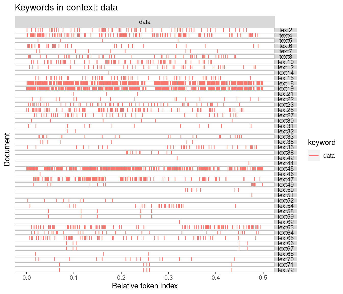

(#fig:kwic_xray)quanteda xray plot - 1

The following xray plot shows the frequency of usage of the keywords ‘data’, ‘personal’, and ‘localization’ across the corpus.

kwic1 <- kwic(tokens1_ngram, c('data', 'personal', 'localization'))
#head(kwic1)

textplot_xray(kwic1) + aes(color = keyword) + ggtitle(paste('Keywords in context:', 'data, personal, localization'))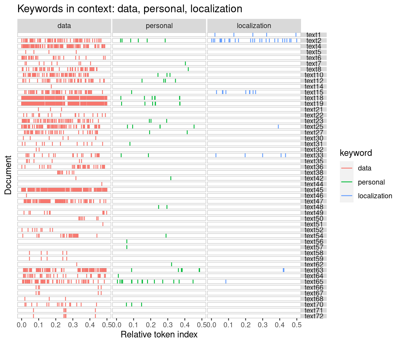

(#fig:kwic_xray2)quanteda xray plot - 2

#png("xray_textplot_kwic.png", width=800, height=800)
#textplot_xray(kwic1) + aes(color = keyword) + ggtitle(paste('Keywords in context:', 'data, personal, localization'))
#dev.off()

4.2 Frequency of terms and the document-feature matrix

A basic aspect of content analysis is to assess the importance of terms or features by computing their frequency of usage. This allows the identification of “important” terms in the corpus and it also may be used to assess whether keywords selected for analysis using keywords-in-context are important in the corpus. A further step (later in this exercise) is to assess how terms are related to one another (part of this would involve assessing how keywords studied using keywords-in-context are related other terms in the corpus).

To answer these questions we first create a document-feature matrix. Note the shift in terminology. In setting up the corpus, we talk about tokens. Now that the cleaning, simplification and standardisation is done, we talk about features (remember that in this blogpost we use ‘terms’ and ‘features’ interchangeably). Below we print the top-10 features (based on frequency) and we plot a word cloud of the 200 most frequently-used features.

dfm1  <-  dfm(tokens1_ngram)
dfm1 %>% topfeatures(10) %>% kable()

	x
data	2906
|	984
indigenous	807
health	427
research	378
can	369
sovereignty	346
access	346
services	337
ids	336

textplot_wordcloud(dfm1, min_size = 1, max_words = 200)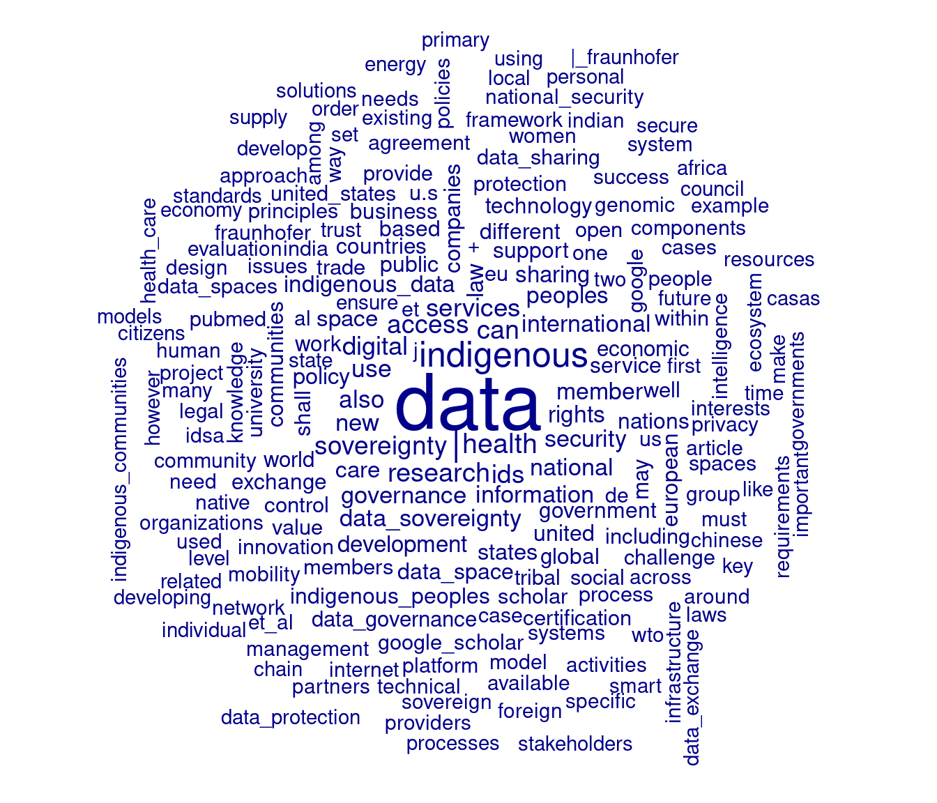

Figure 1: Word cloud

As we found in the previous post where we produced a word cloud produced with the tidytext and wordcloud packages, the word cloud is dominated by the presence of the word ‘data’. In the previous post, we used a customised stop word list to remove ‘data’ from the word cloud. In the present post, we will control for the dominance of the word ‘data’ using another approach. Specifically, we will make use of the term frequency-inverse document frequency (tf-idf) weighting scheme, which weight counts of features according to the how often they appear in that document vs. how many documents contain that feature. The tf-idf weighting scheme can often give a better sense of significance of a keyword in a document and a corpus. In the following code, we also use the tokens_select() function in quanteda to remove tokens that have fewer than three characters in length (this will remove the pipe character “|”, which is presently the second-ranked feature in terms of frequency of use).

dfm1 <- tokens1_ngram %>% tokens_select(min_nchar = 3) %>% dfm()
dfm1 %>% dfm_tfidf() %>% topfeatures(10) %>% kable()

	x
data	565.4340
indigenous	466.9132
ids	463.7510
health	247.0532
data_space	210.8858
google_scholar	197.6504
indigenous_data	179.1825
pubmed	174.3059
fraunhofer	168.0807
scholar	161.9302

dfm1 %>% dfm_tfidf() %>% textplot_wordcloud(min_size = 1, max_words = 200)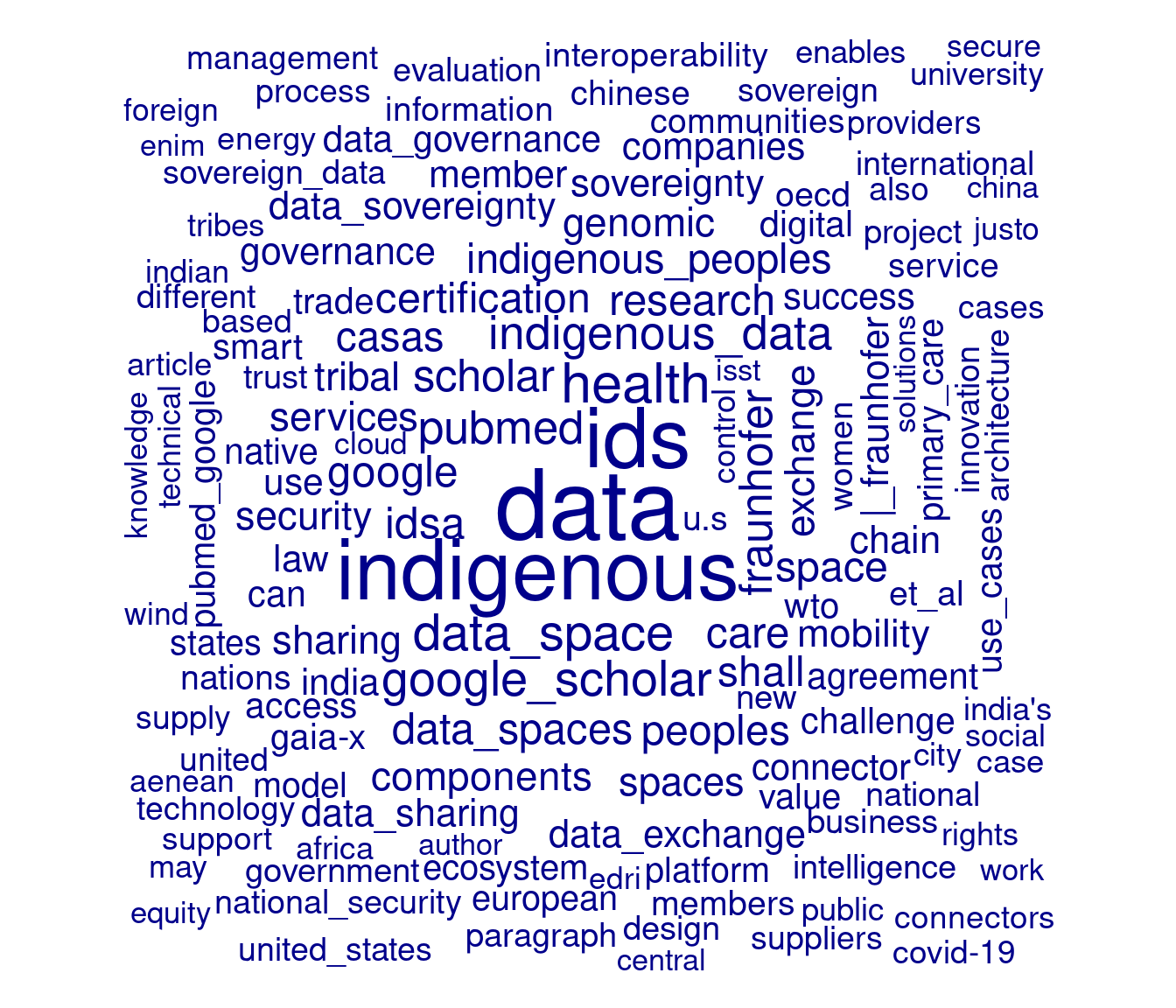

Figure 2: Word cloud - 2

4.3 Using dictionary-based coding

Creating a dictionary is one way to code documents according to a specific set of questions or problems. A dictionary can also be used to handle synonyms.

dict1  <-  dictionary(list(identity = c('identity', 'identities', 'ids'),
                                member = c('member', 'members')))

tokens2  <-  tokens_lookup(tokens1_ngram,
    dictionary = dict1,  exclusive = FALSE)

dfm2 <- tokens2 %>% tokens_select(min_nchar = 3) %>% dfm()
dfm2 %>% dfm_tfidf() %>% topfeatures(10) %>% kable()

	x
data	565.4340
indigenous	466.9132
health	247.0532
identity	245.0384
data_space	210.8858
google_scholar	197.6504
indigenous_data	179.1825
pubmed	174.3059
fraunhofer	168.0807
scholar	161.9302

dfm2 %>% dfm_tfidf() %>% textplot_wordcloud(min_size = 1, max_words = 200)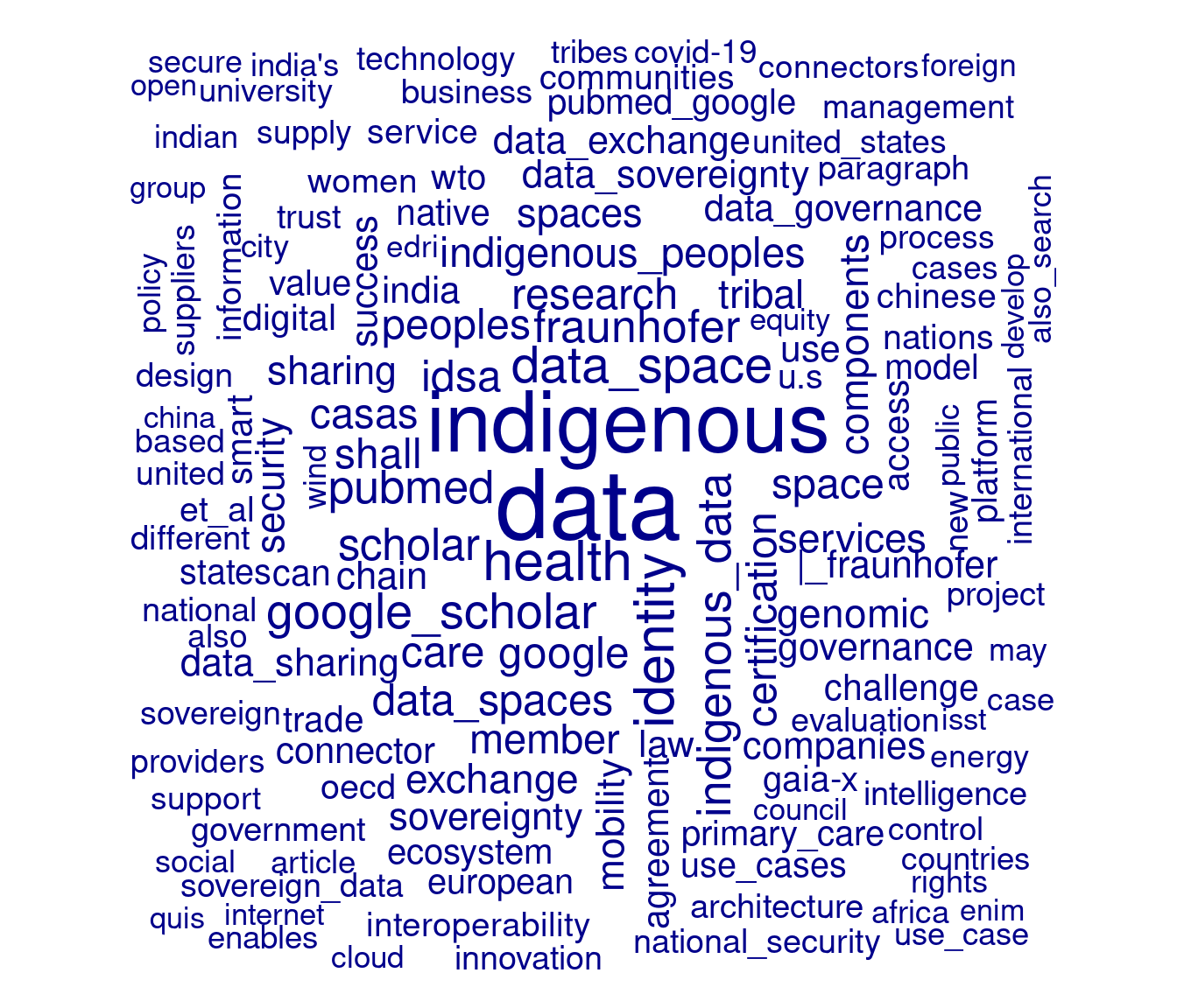

Figure 3: Word cloud - 3

With the use of the above dictionary, we find that ‘health’ becomes the third-top feature (when using the tf-idf weighting) and ‘identity’ moves to fourth. While we do not examine this here, by setting exclusive=FALSE in tokens_lookup() we can reduce the corpus to only those terms in the dictionary. A dictionary might cover several themes, or you might have separate dictionaries for each theme.

4.4 Comparison cloud

As a final step in this blog post, we show how to produce a comparison cloud (comparing word use by organisations from the Global North and Global South) using quanteda.

dfm3 <- dfm2 %>% dfm_group(type) %>% dfm_trim(min_termfreq = 3)
textplot_wordcloud(dfm3, comparison = TRUE, min_size = 1, max_words = 100, color = c("red", "blue"))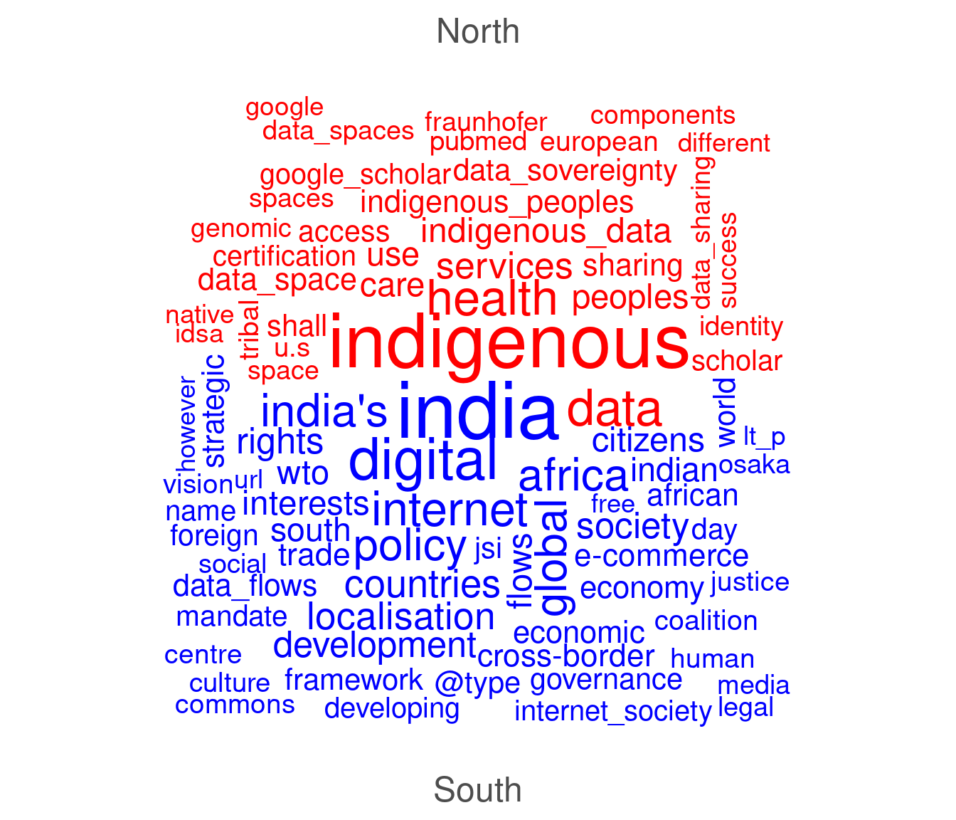

Figure 4: Comparison cloud

The word cloud above compares prominent words and phrases produced by the Global North and the Global South organisations. It appears that indigenous-related issues and health are the most prominent topic in the North. Using quanteda to perform unigram and bigram, it becomes possible to detect themes and a number of potential sub themes such as a topic of ‘indigenousity’ which is discussed in relation to the problem of ‘indigenous data’ and ‘indigenous peoples’ in the North. Other words such as ‘health’ and ‘services’ are also popular which give us an impression that another potential themes discussed could be related to the problem of health services. It can be said that indigenous data sovereignty and health services become two major concerns for organisations in the North when discussing data sovereignty issues.

Meanwhile in the South, the word ‘digital’ and ‘policy’ along with names such as ‘India’, ‘Africa’ and ‘countries’ are interestingly dominant in the discussion. It may indicate that digital policy issues are central for organisations in the South compared at least to the North. Probably, India and African countries inform about the context of where such issues emerged. It is interesting to notice that other potentially meaningful phrases such as ‘right’, ‘development’ and ‘cross-border data flows’ are most frequently discussed in the South. A concept of the North/South divide might provide some clues to answer why organisations in different regions raise different concerns of issues when data sovereignty notions are debated on the web.